
I. What is COSMO-RS ❓#
COSMO-RS (COnductor like Screening MOdel for Real Solvents) is a theoretical approach used to calculate solvation phenomena in chemistry 1. It provides a way to estimate the thermodynamic properties of fluid systems based solely on the molecular structure. It predicts how a solvent will behave and interact with a solute being capable of estimating different thermodynamic metrics such as partition coefficients, solvation energies and the sigma profiles have been used to correlate and predict successfully many properties including density, surface tension, and vapor pressure 3,1,2.
A bit of history 📜#
The computational description of molecules in the fluid phase represented a challenge, for the current methods at the time struggled to capture the complex interactions between the molecules like polarization effects and cooperative interactions.
In the 1970s, research concentrated on treating the solvent as a continuous medium surrounding the molecule. The models in use employed a concept known as ‘dielectric theory’, which helps to understand how the solvent’s electric field influences the solute. These models are called SCRF (self-consistent reaction field), and they create a boundary around the solute to simulate the solvent’s effect, similar to the image below:

The iterative process is to calculate how the solvent’s electric field changed due to the solute and then adjusting until consistency is reached. This is defined as the stable state where the solute’s properties remain constant and do not change upon additional calculations.
COSMO-RS comes into play 🎲#
In the case of COSMO-RS the COSMO (COnductor like Screening MOdel) model 3,1,2 is used to determine the dielectric screening charges and energies, using a surface around the molecule which, depending on the quantum chemical package used, can resemble the van der Waals or vdW surface. This surface is like the intersection volume of a sphere on every atom with a specific radius that outlines the shape of a molecule.
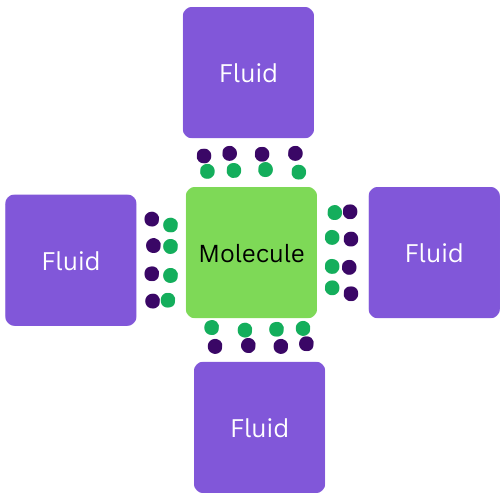
Screening means that the electric fields are counteracted, resulting in no net electric field. Therefore, instead of viewing fluids as interacting through complex fields, they are visualized as ideally screened. In the 1995 paper written by Andreas Klamt, it shows a perfectly screened molecule, like the image below, where the purple and green points (representing the electrons) perfectly cancel each other.
The σ-profiles 📊#
However, real molecules do not have “flat faces”, so a new concept called effective segment area is introduced, which are portions of the molecule’s surface used to approximate interactions. This size is generally fitted to thermodynamic data.
Each segment has a uniform surface charge density - so it can be represented as an average charge density of the area it covers. The number of possible contacts \(n_{x}\) is calculated using the screening area \(A_x\) , which is the total surface involved in interacting with the solvent, and the effective segment area \(A_eff = \pi*Reff^2 \), where \(R_{eff}\) is the effective segment radius. Klamt specifies that an effective segment radius of 1 Å (angstrom) works well 1. The formula is:
\(n_{x} =A_x/A_eff \)
By averaging the surface charge densities over typical contact segments of molecules some peaks of the charge density can be smoothed. Additionally, we can obtain a probability function \(p_x(\sigma)\) i.e. σ-profile, which is like a histogram that shows the distribution of the screening charge density over the molecule’s surface. For solvents that contain mulitple components, the σ-profile is the weighted sum of the component’s profiles:
\(p_S(\sigma) = \Sigma x_i n^x_i p^X_i(\sigma) / \Sigma x_in^x_i \)
where:
\(x_i\) is our molar concentration
\(n^x\) is the contact segment
\(p^X_i(\sigma)\) is the effective probability function, which calculates the probability of finding an average \(\sigma\) on a typical contact segment
Real fluids vs ideal ones 💧#
As mentioned, fluids are being visualized as ideally screened where two segments with opposite surface charge densities interact perfectly so their net energy is zero. However, with real fluids it is not possible due to entropy and the non-ideal nature of molecular interactions; therefore, they do not cancel perfectly each other’s charges. These non-ideal parings result in a “misfit energy”.
The misfit energy represents the interaction energy of two segments with unequal surface charges. This situation occurs because the solute’s surface segments pair with other surface segments with a charge density that not equal to the opposite of its charge density, resulting in a mismatch or misfit energy that balances the non-ideal screening. The misfit energy quantifies the interaction energy of two segments interacting with radius \(R_{eff}\) and surface charges \(\sigma_1, \sigma_2\). The total misfit energy is the sum of the misfit energies for all of its surface segments:
\(E^x_{mf} = \frac{1}{2} \alpha \Sigma \sigma_\nu^2 = \frac{1}{2} \alpha N^x \int p^x(\sigma)\sigma^2 d\sigma\)
where:
\(\alpha=\frac{1.2\pi^{5/2}R_{eff}^3}{(4\pi\epsilon_0)}\), is constant that scales the interaction energy based on the geometry and properties of the segments
\(\sigma_\nu\) is the averaged screening charge density
\(N^x\) is the total number of effective surface segments.
The way the surface segments are arranged is limited by the shapes of the molecules. However, COSMO-RS simplifies the calculations by ignoring these constraints. This means that the segments are treated as if they can pair freely, a concept known as decoupling.This means we can think of the liquid as being made up of N parts, each with their own surface charge density, \(\sigma\). The lowest possible misfit energy (“ground state”) \(E_s^{GS}\) is reached when segments are paired such that the sum \(\sigma_{+i} + \sigma_{−i}\)) is minimised:
\(E_s^{GS} = \frac{1}{2}\alpha'\sum_{i=1}^{N/2}(\sigma_{+i} + \sigma_{-i})^2\)
The value of the misfit energy of the ground state tells us how good a fluid is at screening its own molecules; therefore, the lower the misfit energy, the better the screening.
What is openCOSMO-RS ❓#
This model improves the predictive accuracy of the fluid phase thermodynamics by incorporating multiple segmental descriptors. The screening charge density \(\sigma\) is still the main descriptor, but additional ones such as the polarity counterpart screening charge density introduced by Andreas Klamt, \(\sigma_⊥\), are now being used to improve the model. 4 It is calculated by the formula below:
\(\sigma⊥ = \sigma_\alpha - 0.816\sigma_\alpha^0 \)
Some additional characteristics of the model:
Open Source: it allows people in the academic community to use, evaluate and develop the model
Extended σ-Profile Generation: the new algorithm includes multiple segment descriptors in addition to the screening charge density, as mentioned above.
RDKit/ORCA Workflow: It uses RDKit to generate conformers and ORCA for quantum chemical calculations, which makes it easier for more academic users to implement
Correction to the screening charge correlation: this correction involves an additional descriptor, denoted as σ⊥, which is derived from the screening charge density. This descriptor is used to refine the electrostatic interaction energy calculations. In a molecule, the electrostatic forces play a crucial role in determining how molecules interact with each other - the charge in one area can influence the charge in another area and determine if molecules will come together or move apart
More information about its implementation can be found here.
openCOSMO-RS 24a 💫#
The openCOSMO-RS 24a is a new and improved version of the open-source COSMO-RS model. This version is designed to predict solvation free energies using quantum chemical calculations from ORCA 5.
What is the solvation free energy, ΔGsolv? ⚡#
It is the amount of energy involved when a solute dissolves from the gas phase into a solvent. It is the energy change that occurs when the particles of the solute are surrounded and stabilized by the solvent molecules. It is a contributing factor in predicting how substances will behave in a solution.
A positive solvation free energy value shows that the process is not energetically favourable. This means that the solute wants to stay in the gas phase, whereas a negative value shows that the process is energetically favourable, meaning that the solute prefers to be in the solvent. The model can calculate this property using the following improvements:
QSPR model: A QSPR model is a way of using a molecule’s structure to predict the molar volumes of the solvents
Gas Calculation The workflow was improved and a gas phase energy calculation was included, using a newer version of ORCA.
More information about this newer version can be found here 5